混合数据同化技术
基本原理
基于美国国家环境预报中心(NCEP)的业务快速同化循环更新预报系统(Rapid Refresh,即RAP)以及业务高分辨率快速同化循环更新预报系统 (High-Resolution Rapid Refresh,即HRRR),我们设计出一套高分辨率快速同化循环更新预报系统(RAP和HRRR)以满足短临精细化预报的服务要求。该系统采用的是目前国际上流行的混合数据同化方案,使用的是美国NCAR的WRFDA系统,或者NCEP的业务数据同化系GSI。
区别于传统的数据同化技术,混合同化是将变分同化和集合卡尔曼滤波有机的耦合在一起,实现他们相互间的优势互补与局限性减弱,从而可以最优化地和最大限度地使用各种现有常规和非常规气象观测数据(地面、探空、自动站、风廓线、多普勒雷达、地基GPS-MET和卫星等)。针对不同观测数据,混合同化技术根据实时大气环流信息以及各种物理平衡条件,为短临天气预报模型提供一个最优化的初始条件,从而进一步提升模式预报结果的准确度。另外,根据观测数据的实时传输情况,混合同化技术可以将最新的数据引入预报模式,从而提供不断更新的短期临近预报结果。
对于一般的变分同化而言,其可以描述为对目标泛函 \(J\) 进行收敛,从而获得对天气预报的初试场 \(x\) 的最优分析。目标泛函 \(J\) 的增量(incremental)表述形式为:
\[J = \frac{1}{2} \delta x_0^\intercal \mathrm{B}^{-1} \delta x_0 + \frac{1}{2} \sum_{k=0}^K (\mathrm{H}_k \mathrm{M}_k \delta x_0 - d_k)^\intercal \mathrm{O}^{-1} (\mathrm{H}_k \mathrm{M}_k \delta x_0 - d_k) + J_c\]以上方程可以转换为控制变量表述的形式,使用
\[\delta x_0 = \mathrm{U} v \; , \; \mathrm{B} = \mathrm{U} \mathrm{U}^\intercal\]\[J = \frac{1}{2} v^\intercal v + \frac{1}{2} \sum_{k=0}^K {(\mathrm{H}_k \mathrm{M}_k \mathrm{U}_k v - d_k)^\intercal \mathrm{O}^{-1} (\mathrm{H}_k \mathrm{M}_k \mathrm{U}_k v - d_k)} + J_c\]
同理,另外一种优化方法“集合卡曼滤波”(EnKF),其本质上和变分方法具有一致性,只是方式不同,EnKF使用了一个预报集合对当前大气环流场的不确定性进行显性的估计,从而建立对背景场误差协方差矩阵的近似分析,从而对收敛函数的下降方向给出直接迭代关系:
\[x^a = x^f + \mathrm{K} d \; , \; \mathrm{P}^f \approx \overline{x^f (x^f)^\intercal} = \frac{1}{N-1} \sum_{i=1}^N {(x_i^f - \overline{x^f}) (x_i^f - \overline{x^f})^\intercal}\]\[\mathrm{K} = \mathrm{P}^f \mathrm{H}^\intercal (\mathrm{H} \mathrm{P}^f \mathrm{H}^\intercal + \mathrm{O})^{-1}\]混合数据同化实际上是将变分方法和EnKF进行结合,汲取两者之长,从而解决它们自身的弱点。简而言之,我们可以理解为将EnKF中的背景场误差协方差矩阵引入到目标泛函的收敛过程中,从而加入集合预报当前环流场信息到优化方程的收敛过程中:
\[J_b = J_b1 + J_b2 = \frac{1}{2} \delta x_0^\intercal [(1-\beta) \mathrm{B} + \beta \mathrm{P}_0^f \circ \mathrm{C}]^{-1} \delta x_0\]其中 \(P^f\) 就来源于EnKF。然而,为了可以进行计算和迭代求解,我们需要对以上方程进行改写,并引入转换项(Alpha-Control Transform):
\[\delta x_0 = \delta x_{nmc} + \delta x_{ens} = \mathrm{U} v + \mathrm{X}^f \circ \alpha\]这样一来经过Schur项的背景场误差协方差矩阵局地化空间分析(Covariance Localization),目标泛函的收敛方程及变为:
\[\begin{split}J = \frac{1}{1-\beta} (\frac{1}{2}v^\intercal v) + \frac{1}{\beta} [ \frac{1}{2} \alpha^\intercal \begin{pmatrix} C & & 0 \\ & ... & \\ 0 & & C \end{pmatrix} \alpha ] + \frac{1}{2} \sum_{k=0}^K{(\mathrm{H}_k \mathrm{M}_k \delta x_0 - d_k)^\intercal \mathrm{O}^{-1} (\mathrm{H}_k \mathrm{M}_k \delta x_0 - d_k)} + J_c\end{split}\]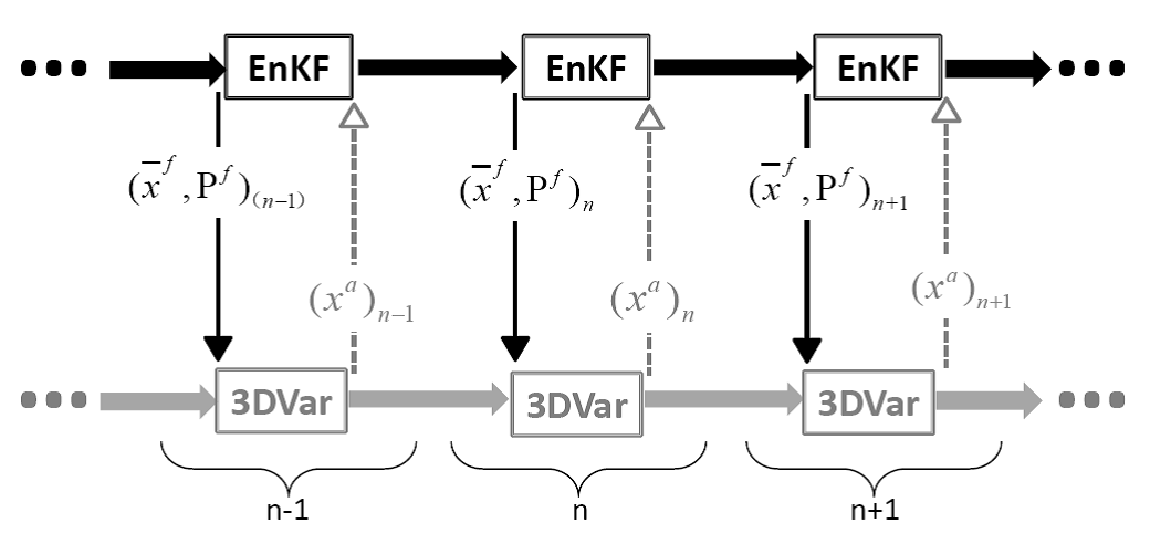
EnKF-3DVar Hybrid 混合数据同化示意图
本项目混合同化部分,可使用NCAR的WRFDA系统,也可以选用美国NCEP的业务数据同化系统GSI,相对于WRFDA系统,GSI系统具有如下几点优点:
- GSI是美国海洋大气局NOAA当前稳定运行的先进业务模式,性能稳定,效果经得起考验;
- 在业务环境下经过多年的磨练,GSI本身对观测资料也有很完善的质量控制;
- GSI功能比较齐全,对几乎所有观测类型都可以同化;
- GSI的混合数据同化已经在全球预报(GFS)和区域高分辨率模式中(RAP和HRRR)业务化运行;
- GSI具备3DVar和4DVar的功能,可以结合EnKF部分实现三维和四维的混合同化。
单点试验
WRFDA的混合资料同化的单点试验
在模式21层放入一个位温的单点观测,进行同化,观测不同的背景误差协方差矩阵对分析增量的影响,如下图:
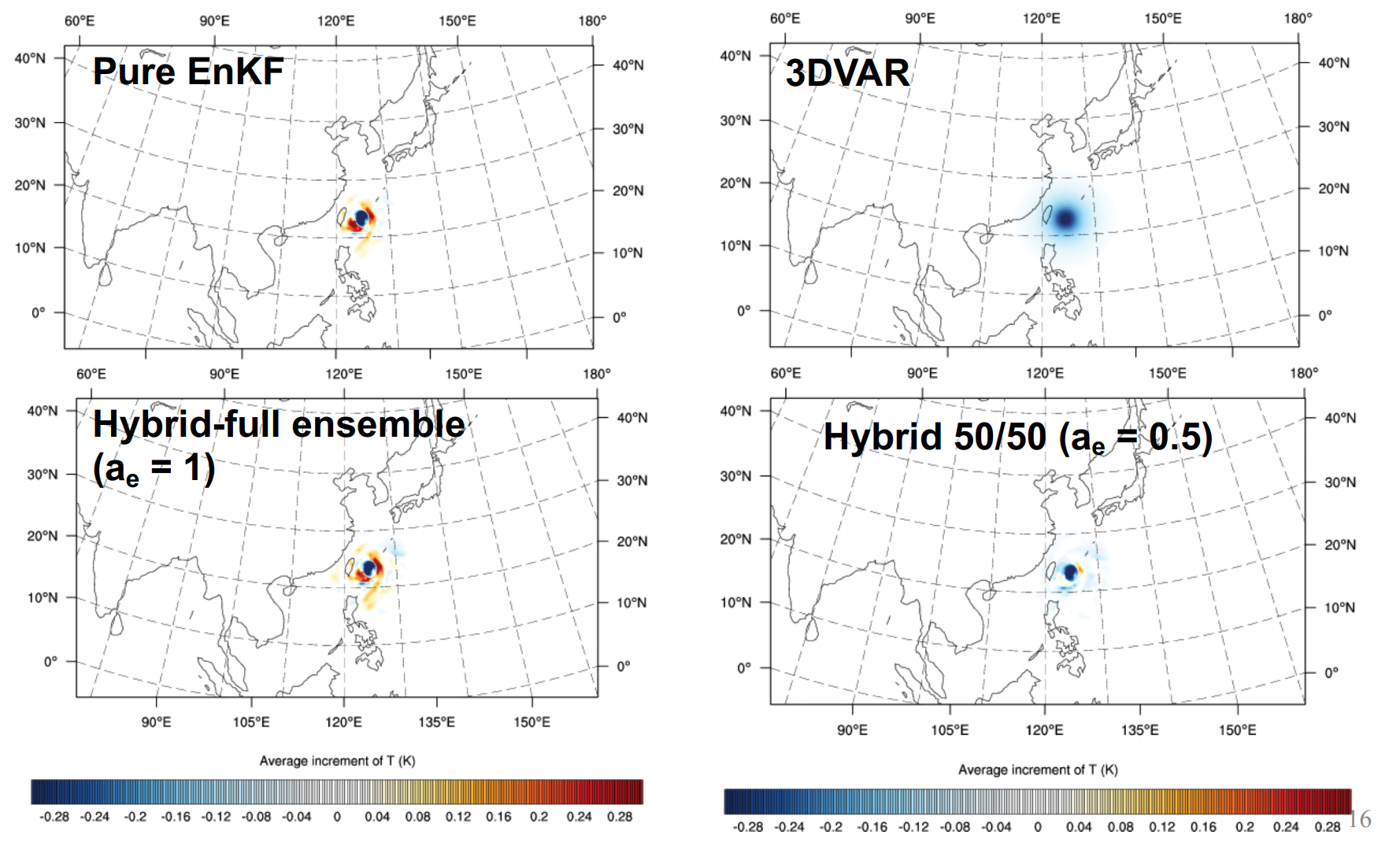
上图显示了四种情形:
- 集合卡尔曼滤波给出的分析增量(Pure EnKF)
- 背景误差协方差矩阵使用WRFDA系统的静态B矩阵(3DVar)
- 背景误差协方差矩阵完全由集合预报给出(Hybrid full-ensemble)
- 背景误差协方差矩阵50%来自集合预报,50%来自静态B(Hybrid 50/50)
具体应该使用什么样的比例,不在此讨论,应该运行大量研究作业来确定。
GSI的混合资料同化的单点试验
沈阳大气所每日实时下载美国NCEP的20个集合预报成员,我们利用这20个集合成员计算背景误差协方差矩阵的集合部分。理论上,RAP混合资料同化方法需要40个以上的集合预报成员,由于下载带宽的限制,暂且使用20个集合成员。
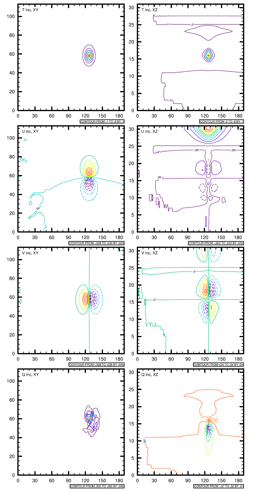
为了测试静态背景误差协方差矩阵和混合背景误差协方差矩阵的差别,我们选取单点试验的方法,来显示背景误差协方差矩阵对单个观测的作用。具体方法是在模式区域中间放置一个500hPa的观测,例如:温度观测,其和背景场的差为2度,假设其观测误差为0.1,分别使用静态的背景误差协方差矩阵和混合背景误差协方差矩阵,运行3DVar,画出其分析增量图,该增量图为背景误差协方差矩阵的物理表达。
 |
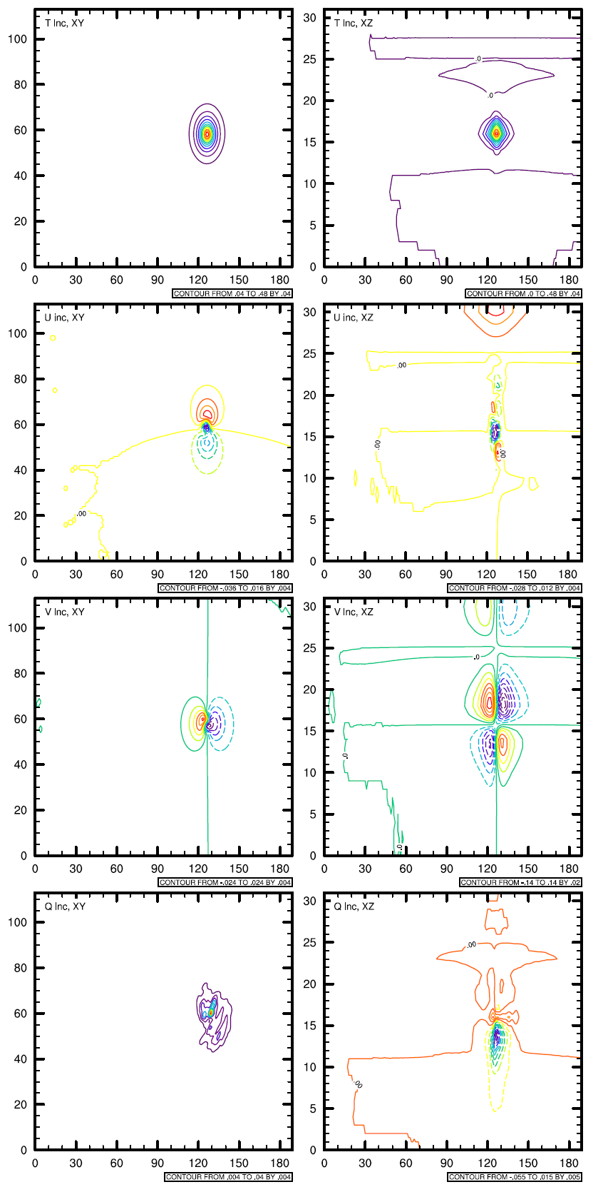 |
上图从上到下分别为:
- 水平方向500hPa,温度场的分析增量;XZ垂直剖面的温度分析增量
- 水平方向500hPa,东西方向风场的分析增量;XZ垂直剖面的东西方向风场分析增量
- 水平方向500hPa,南北方向风场的分析增量;XZ垂直剖面的南北方向风场分析增量
- 水平方向500hPa,水汽风场的分析增量;XZ垂直剖面的水汽场分析增量
可以看到:使用了集合信息的混合背景误差协方差矩阵所产生的分析增量与使用静态背景误差协方差矩阵产生的分析增量的不同,尽管从物理上,无法解释它们之间的差别,但我们可以认为混合资料同化加入了流依赖的信息,即:the error of the day.
具体实施
WRFDA的实施细节
The procedure is the same as running 3DVAR, with the exception of some extra input files and namelist settings. The basic input files for WRFDA are LANDUSE.TBL, ob.ascii or ob.bufr (depending on which observation format you use), and be.dat (static background errors). Additional input files required for 3DEnVar are a single ensemble mean file (used as the fg for the hybrid application) and a set of ensemble perturbation files (used to represent flow-dependent background errors).
A set of initial ensemble members must be prepared before the hybrid application can be started. The ensemble can be obtained from other ensemble model outputs, or you can generate them yourself. This can be done, for example, adding random noise to the initial conditions at a previous time and integrating each member to the desired time. A tutorial case with a test ensemble can be found at Tutorial . In this example, the ensemble forecasts were initialized at 2015102612 and valid 2015102712. A hybrid analysis at 2015102712 will be performed using the ensemble valid 2015102712 as input. Once you have the initial ensemble, the ensemble mean and perturbations can be calculated following the steps below:
Set an environment variable for your working directory and your data directory
> setenv WORK_DIR your_hybrid_path
> setenv DAT_DIR your_data_path
> cd $WORK_DIR
Calculate the ensemble mean
From your working directory, copy or link the ensemble forecasts to your working directory. The ensemble members are identified by the characters
.e###at the end of the file name, where###represents three-digit numbers following the valid time.> ln –sf $DAT_DIR/Hybrid/fc/2015102612/wrfout_d01_2015-10-27_12:00:00.e* .Provide two template files (ensemble mean and variance files) in your working directory. These files will be overwritten with the ensemble mean and variance as discussed below.
> cp $DAT_DIR/Hybrid/fc/2015102612/wrfout_d01_2015-10-27_12:00:00.e001 ./wrfout_d01_2015-10-27_12:00:00.mean
> cp $DAT_DIR/Hybrid/fc/2015102612/wrfout_d01_2015-10-27_12:00:00.e001 ./wrfout_d01_2015-10-27_12:00:00.vari
Copy
gen_be_ensmean_nl.nl(cp $DAT_DIR/Hybrid/gen_be_ensmean_nl.nl .) You will need to set the information in this script as follows:&gen_be_ensmean_nl directory = '.' filename = 'wrfout_d01_2015-10-27_12:00:00' num_members = 10 nv = 7 cv = 'U', 'V', 'W', 'PH', 'T', 'MU', 'QVAPOR' /
where directory is the folder containing the ensemble members and template files, filename is the name of the files before their suffixes (e.g.,
.mean,.vari, etc),num_membersis the number of ensemble members you are using,nvis the number of variables, andcvis the name of variables used in the hybrid system. Be surenvandcvare consistent!Link
gen_be_ensmean.exeto your working directory and run it.> ln –sf $WRFDA_DIR/var/build/gen_be_ensmean.exe . > ./gen_be_ensmean.exeCheck the output files.
wrfout_d01_2015-10-27_12:00:00.meanis the ensemble mean;wrfout_d01_2015-10-27_12:00:00.variis the ensemble variance
Calculate ensemble perturbations
Create a sub-directory in which you will be working to create ensemble perturbations.
> mkdir –p ./ep
> cd ./ep
Run
gen_be_ep2.exe. The executable requires four command-line arguments (DATE, NUM_MEMBER, DIRECTORY, and FILENAME) as shown below for the tutorial example:> ln –sf $WRFDA_DIR/var/build/gen_be_ep2.exe . > ./gen_be_ep2.exe 2015102712 10 . ../wrfout_d01_2015-10-27_12:00:00
Check the output files. A list of binary files should now exist. Among them,
tmp.e*are temporary scratch files that can be removed.
Back in the working directory, create the input file for vertical localization. This program requires one command-line argument: the number of vertical levels of the model configuration (same value as
e_vertin the namelist; for the tutorial example, this should be 42).> cd $WORK_DIR > ln –sf $WRFDA_DIR/var/build/gen_be_vertloc.exe . > ./gen_be_vertloc.exe 42
The output is
./be.vertloc.datin your working directory.Run WRFDA in hybrid mode
In your hybrid working directory, link all the necessary files and directories as follows:
> ln -fs ./wrfout_d01_2015-10-27_12:00:00.mean ./fg  (first guess is the ensemble mean for this test case)
> ln -fs $WRFDA_DIR/run/LANDUSE.TBL .
> ln -fs $DAT_DIR/Hybrid/ob/2015102712/ob.ascii ./ob.ascii
> ln -fs $DAT_DIR/Hybrid/be/be.dat ./be.dat
> ln –fs $WRFDA_DIR/var/build/da_wrfvar.exe .
> cp $DAT_DIR/Hybrid/namelist.input .
Edit
namelist.input, paying special attention to the following hybrid-related settings:&wrfvar7 je_factor = 2.0 / &wrfvar16 ensdim_alpha = 10 alphacv_method = 2 alpha_corr_type=3 alpha_corr_scale = 500.0 alpha_std_dev=1.000 alpha_vertloc = .true. /
Finally, execute the
da_wrfvar.exe, running in hybrid modeCheck the output files; the output file lists are the same as when you run WRF 3D-Var.
GSI的实施细节
将集合预报的产品,插值到预报网格上,并计算所需要的集合信息
所使用的程序代码位于:
/sya/u/gongying/LongRun/nwprod/rap.v2.0.11/sorc/rap_process_enkf.fd
使用混合背景误差协方差矩阵进行变分资料同化
所使用的代码位于:
/sya/u/gongying/LongRun/nwprod/rap.v2.0.11/sorc/rap_gsi.fd
需要注意的参数有:
- Set the location of the ensemble files in the variable
ENS_ROOT=… - Set to run GSI hybrid analysis:
if_hybrid=Yes - Set not to run GSI 4D hybrid analysis:
if_4DEnVar=No
- Set the location of the ensemble files in the variable